Venture Capital (VC) and Raising Funds
Overview of how VC fits into the broader financial ecosystem
- An important reminder!
- Another announcement!
Prepare
📖 Read Alternative Investment Book, Sec 8.1: Venture Capital (VC) and Raising Funds
Lecture Slides
Problem Set
Multi-Media: Documentaries, Case Studies, Extra
Something Ventured: A 2011 documentary film about the emergence of American venture capitalism in the mid-20th century. It follows the stories of the venture capitalists who worked with entrepreneurs to start and build companies like Apple, Intel, Genentech, Cisco, Atari, Tandem, and others.
Book of the week:
The Business of Venture Capital by Mahendra Ramsinghani
Application: Event Studies and Futures Markets (Commodities Futures)
Event studies are a statistical method used to assess the impact of a specific event on the value of a firm or market or any other particular interest. This technique is widely used in finance and economics to analyze how market prices respond to an event, such as merger announcements, earnings reports, regulatory changes, or macroeconomic news. The core idea behind event studies is to observe the behavior of stock prices (any action) before and after the occurrence of the event to determine whether there is an abnormal return attributable to the event itself, separating this effect from overall market movements or random fluctuations in stock prices.
The methodology of an event study involves several key steps:
Event Identification: Clearly define the event of interest and the timeframe during which the event is expected to have an impact on stock prices.
Selection of Event Window: Choose an appropriate time period around the event date to analyze the stock’s performance. This includes a pre-event window to capture the stock’s behavior before the event and a post-event window to capture the effect after the event.
Estimation Window: Select a period before the event window to estimate the normal return of the stock, which is the return expected in the absence of the event. This helps in isolating the effect of the event from other factors affecting the stock price.
Calculation of Abnormal Returns (AR): Compute the difference between the actual return observed during the event window and the normal return expected if the event had not occurred. This measures the impact of the event.
Aggregation of Abnormal Returns: Aggregate the abnormal returns over the event window to get the cumulative abnormal return (CAR), which provides a more comprehensive picture of the event’s impact over time.
Statistical Analysis: Conduct statistical tests to determine whether the observed abnormal returns are significantly different from zero, indicating that the event had a statistically significant effect on the stock price.
Event studies are valuable for understanding the efficiency of markets in processing information, the economic impact of events on firms, and for policy analysis. They can provide insights into how different types of events influence investor perception and market value of companies.
The Importance of High-frequency Data
A system of two simultaneous structural equations that affect each other.
\[ \Delta i_{t} = \beta \Delta r_{t} + \gamma z_{t}+ \epsilon_{t} \quad \quad \quad (1) \]
\[ \Delta r_{t} = \alpha \Delta i_{t} + \delta z_{t}+ \eta_{t} \quad \quad \quad (2) \]
- Equation-1 denotes a monetary policy response function which is the response of policy to change in a set of other variables \(z_{t}\) and to the financial asset price \(r_{t}\).
- Equation-2 is the financial asset price equation, that illustrates the asset price to be influenced by the FOMC announcements, \(i_{t}\) and also by the other variables, \(z_{t}\).
- Lastly, \(\epsilon_{t}\) and \(\eta_{t}\) are uncorrelated error terms.
- However, Equation-1 and 2 cannot be estimated consistently since \(\Delta i_{t}\) and \(\Delta r_{t}\) are simultaneously determined in the system.
\[ \begin{align} \begin{pmatrix} 1 & -\beta\\ -\alpha & 1 \end{pmatrix} \begin{pmatrix} \Delta i_{t} \\ \Delta r_{t} \end{pmatrix} = \begin{pmatrix} \gamma \\ \delta \end{pmatrix} z_{t} + \begin{pmatrix} \epsilon_{t} \\ \eta_{t} \end{pmatrix} z_{t} \quad \quad \quad (3) \end{align} \]
Equation-3 is tht matrix form of equation 1 and 2. Having solved, one can obtain the reduced-form solution of the system:
\[ \begin{align} \begin{pmatrix} \Delta i_{t} \\ \Delta r_{t} \end{pmatrix} = \frac{1}{1-\alpha \beta } \left \{ \begin{pmatrix} \beta \delta + \gamma \\ \alpha \gamma + \delta \end{pmatrix} z_{t} + \begin{pmatrix} 1 \\ \alpha \end{pmatrix}\epsilon_{t} + \begin{pmatrix} \beta \\ 1 \end{pmatrix}\eta_{t} \right \} \quad \quad \quad (4) \end{align} \]
Let denote \(\sigma^{2}_{\epsilon}\) is for the variance of MP shock, \(\sigma^{2}_{\eta}\) and \(\sigma^{2}_{z}\) are for the variance of asset price shocks and other shocks. The OLS estimate:
\[ \begin{align} \hat \alpha_{OLS} = \frac{Cov(\Delta i_{t}, \Delta r_{t}) } {Var(\Delta i_{t}) } = \frac{(\beta \delta + \gamma)(\alpha \gamma + \delta)\sigma^{2}_{z} + \alpha \sigma^{2}_{\epsilon} + \beta \sigma^{2}_{\eta} }{\beta \delta + \gamma)^2 \sigma^{2}_{z} + \sigma^{2}_{\epsilon} + \beta^2 \sigma^{2}_{\eta} } \quad \quad \quad (5) \end{align} \]
hence, the bias of the OLS estimate could be
\[ \begin{align} \hat \alpha_{OLS}- \alpha = (1-\alpha \beta) \frac{\beta \sigma^{2}_{\eta}+ \delta (\beta \delta + \gamma)\sigma^{2}_{z} }{\sigma^{2}_{\epsilon} + \beta^2 \sigma^{2}_{\eta} + (\beta \delta + \gamma)^2 \sigma^{2}_{z} } \quad \quad \quad (6) \end{align} \]
According to the Equation-6 the OLS estimate is biased due to both
- simultaneity bias - if \(\beta \neq\) 0 and \(\sigma^{2}_{\eta}\) > 0
- omitted variables bias - if \(\gamma \neq\) 0 and \(\sigma^{2}_{z}\) > 0
Graphical Representation:
Daily data:
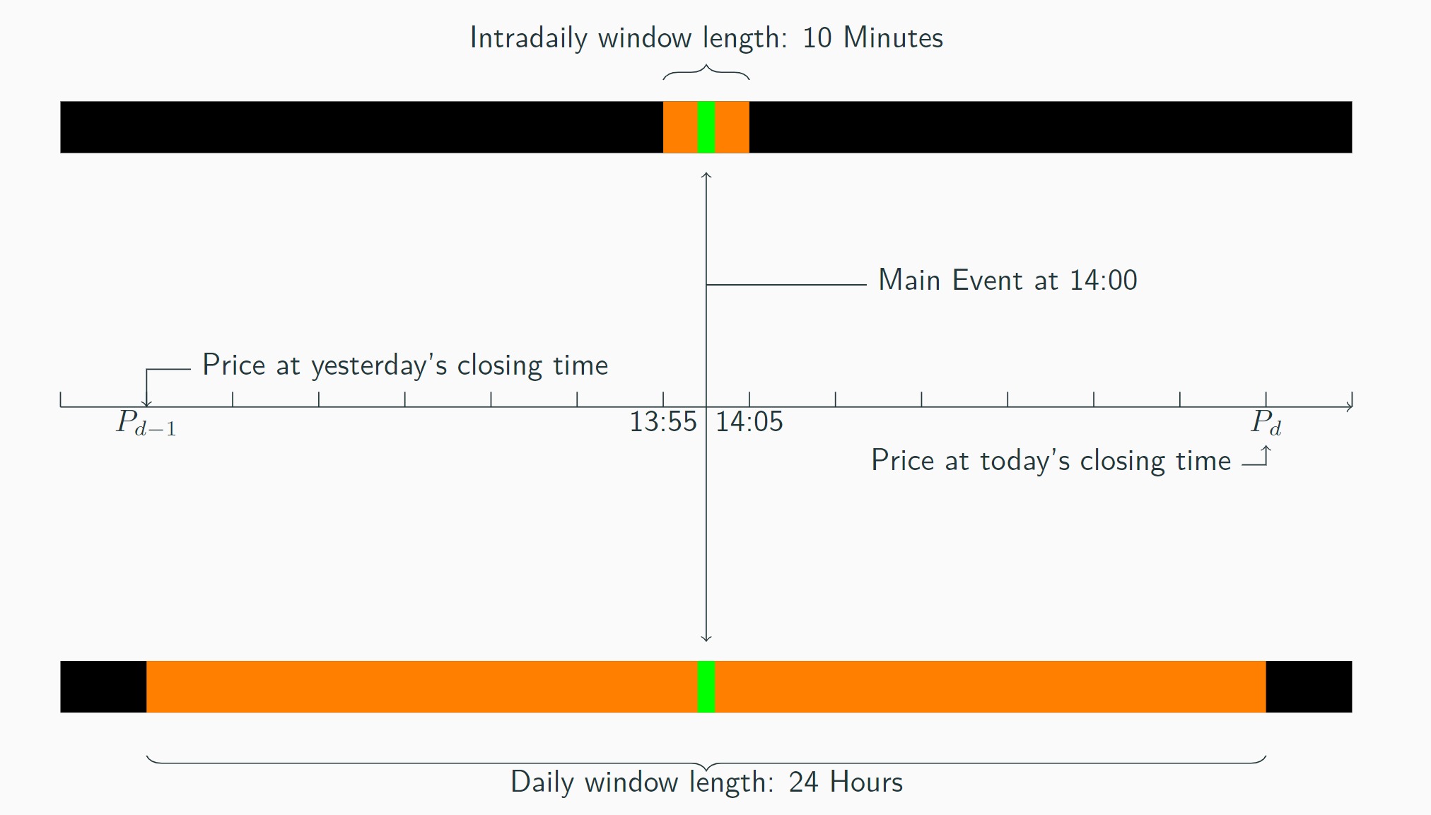
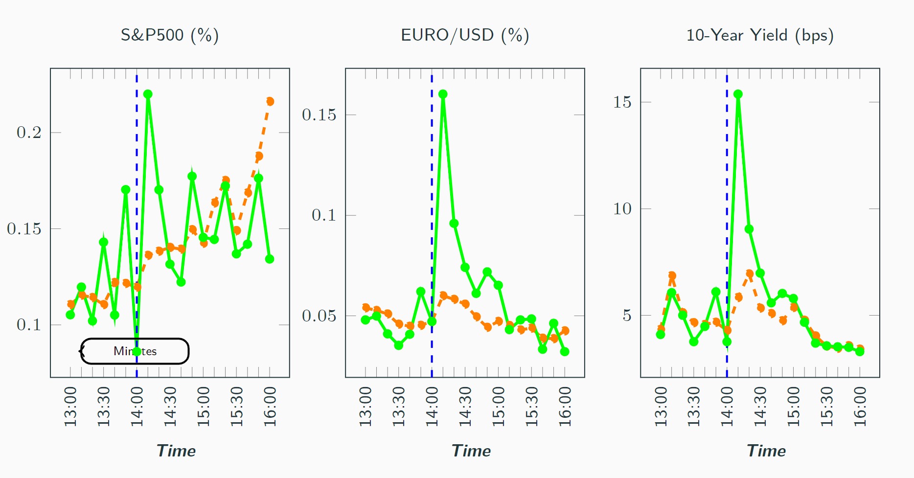
Intradaily data:

An Example from financial markets:
Back to course schedule ⏎